Model Predictive Control in the browser with WebAssembly
If you would like to skip the article, you can:
The demo app does work on mobile, but the experience is improved on a big screen. For some ideas of what to try in the sim, see Interacting with the simulator.

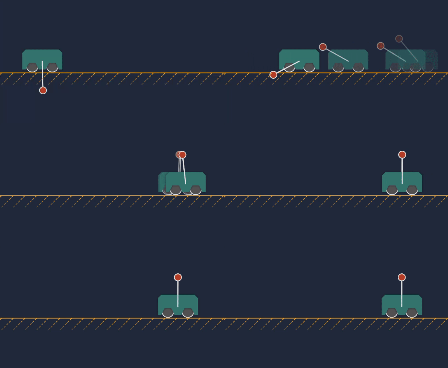
Animation of the cart-pole MPC transitioning from idle to actively controlling the system.
Introduction
First, a caveat: My background is not in control theory, but rather computer vision. The purpose of this project was to improve my practical understanding of trajectory optimization and Model Predictive Control (MPC) by building a working demonstration in simulation. The implementation detailed in this article might be suboptimal in some ways - it is ultimately a toy implementation for my own edification. That said, perhaps it can provide some educational value to others treading the same path.
Additionally, I had been looking for an opportunity to build something with emscripten - a C++ compiler that targets WebAssembly (WASM). Compiling a control algorithm for the browser may seem an unusual choice, but it does afford us some nice properties:
- The final product can be deployed to the web for others to enjoy.
- We can easily connect the algorithm to pretty HTML canvas visualizations and UI elements.
- The iteration time from compilation → visualization is quite fast.
Lastly, the project served as an opportunity to add some new features to wrenfold. wrenfold is a symbolic code-generation framework designed to ease the quick implementation of objective functions for nonlinear optimization problems. (Disclaimer: I am the author of wrenfold).
Problem formulation
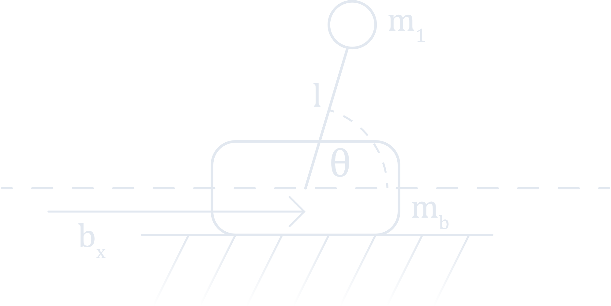
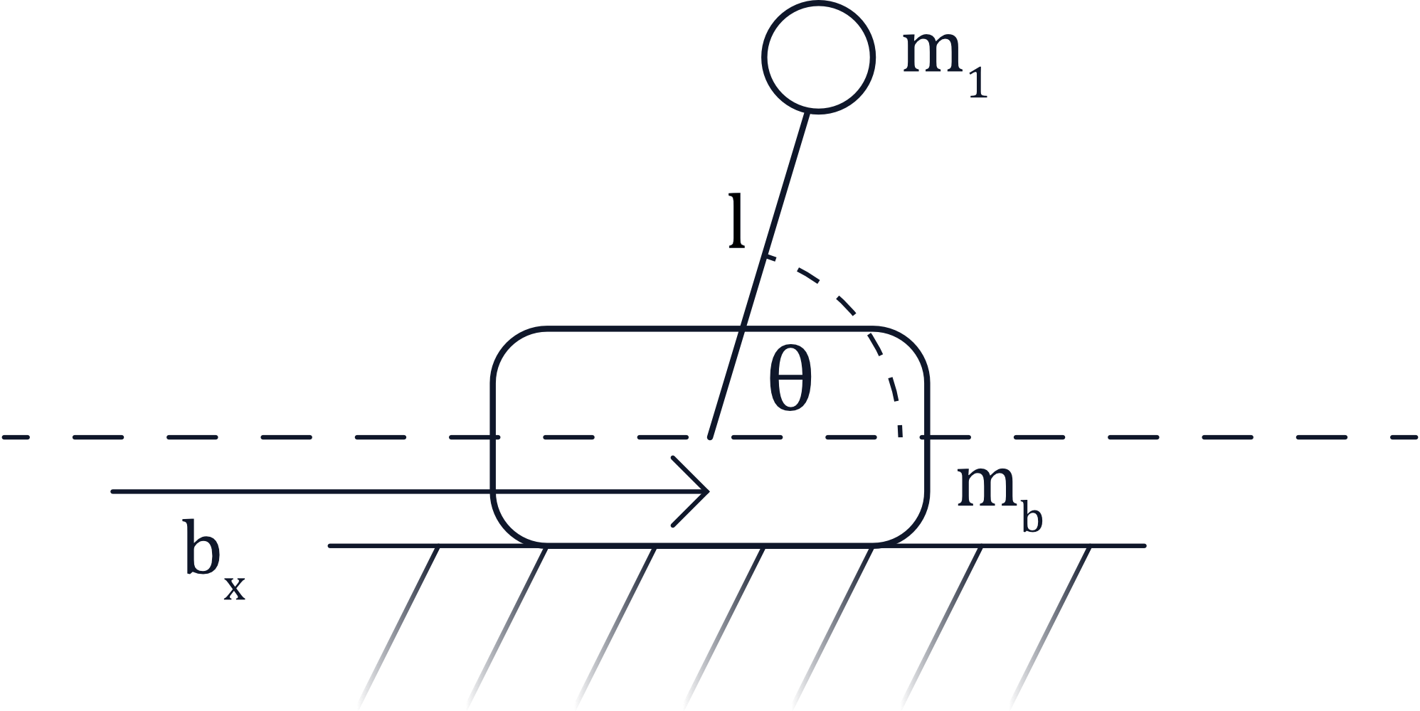
For the sake of simplicity, I selected the cart-pole system to experiment with. The cart-pole consists of a cart or sliding base mass (here denoted $m_b$), atop of which is an inverted pendulum. The pendulum is modeled as a point-mass $m_1$ at the end of an armature of length $l$.


The position of the cart or base along the x-axis is given by $b_x$, and the angle of the pendulum is denoted as $\theta$. The goal of the problem is to stabilize the pendulum in the vertical position (with the selected convention that would correspond to $\theta = \frac{\pi}{2}$). The controller can only apply a lateral force to the base, so we must compute a series of translational control actions that will rotate the pendulum into the desired configuration (a “swing-up” trajectory). Once vertical, we want the system to remain stationary.
Equations of motion
We denote the current state of the system as $\mathbf{x} = \begin{bmatrix}b_x & \theta & \dot{b_x} & \dot{\theta}\end{bmatrix}$. In other words: the base position, pole angle theta, and their respective time derivatives. Our control action on the base is $u$. In order to understand how the system will evolve over time, we must first identify the equations of motion. These equations will yield a function $f$ that describes the rate of change in our state as a function of the current system configuration:
$$\dot{\mathbf{x}} = f\left(\mathbf{x}, u\right)$$
To compute the equations of motion, I formulated the Lagrangian in Python using wrenfold, and employed symbolic differentiation to obtain the Euler-Lagrange equations. The Euler-Lagrange equations can then be rearranged to find $f$. The full derivation is omitted here, but you can read it in code format in the GitHub repo. In addition to the dynamics and control action, I added four additional forces:
- Coulomb friction opposes the motion of the cart. A smoothed model of friction (using the $\tanh$ function) is employed to ensure a continuous derivative.
- The pendulum mass experiences an aerodynamic drag force proportional to speed squared.
- The workspace is bounded on the left and right by two stiff springs that act against the cart if it exceeds some threshold: $|b_x| > x_s$.
- An external force (applied to either the cart or the pendulum mass) is added to model disturbances induced by a human. This is so that the user can click to interact directly with the simulation.
With a symbolic implementation in hand, it is straightforward to code-generate a C++ function that computes $f$ as well as its Jacobians wrt $\mathbf{x}$ and $u$.
MPC optimization problem
Note: For a more complete understanding of this problem, I would advise reading Russ Tedrake’s course notes on trajectory optimization - I found these to be an invaluable resource. Alternatively, Steve Brunton provides a great high-level introduction to the MPC algorithm on his YouTube channel. I will provide a simplified overview and gloss over some of the details.
The equations of motion provide a predictive model that we can integrate forward to determine the system state at some future time. If $t_0$ is the current time and $\mathbf{x}\left(t_0\right)$ is known, we can integrate any hypothetical series of control actions $u(t)$ over a window $[t_0, t_{f}]$ to determine a predicted final state $\mathbf{x}\left(t_f\right)$. The interval between $t_0$ and $t_f$ is the planning horizon.
At a high level, we can then formulate an optimization problem for the control actions $u(t)$ that will result in $\mathbf{x}\left(t_f\right)$ matching some desired terminal $\mathbf{x}_d\left(t_f\right)$. In the case of our cart-pole system, the desired state would be $\mathbf{x}_d\left(t_f\right) = \begin{bmatrix}0 & \frac{\pi}{2} & 0 & 0\end{bmatrix}$ - a stationary cart at the center of the workspace, with the pendulum vertical.
In practice, the system is discretized in time and our control input is represented as a sequence of $N$ actions $\mathbf{u} = \begin{bmatrix}u\left(0\right) & u\left(1\right) & … & u\left(N - 1\right)\end{bmatrix}$ over a bounded window [0, N] rather than a continuous function $u\left(t\right)$. Then we can implement an optimization problem of the form:
$$\DeclareMathOperator*{\argmin}{argmin} \begin{equation} \begin{split} \hat{\mathbf{u}} & = \argmin_{\mathbf{u}} g(\mathbf{u}, \mathbf{x}) \\[5pt] \text{subject to } \mathbf{x}\left[N\right] & = \mathbf{x}_d\left(t_f\right) \end{split} \label{eq:single} \end{equation}$$
Where the values of $\mathbf{x}$ over the window are given by integration:
$$\begin{equation*} \begin{split} \mathbf{x}\left[k + 1\right] & = F\left(\mathbf{x}\left[k\right], u\left[k\right]\right) \\[5pt] \mathbf{x}\left[0\right] & = \mathbf{x}\left(t_0\right) \end{split} \end{equation*}$$
Where $F$ is the discrete integration of the dynamics $f$. The objective function $g$ guides our choice of $\mathbf{u}$ by favoring solutions that achieve some design criteria. For example, we can elect to penalize solutions that introduce large discontinuities between sequential control inputs $u\left[k\right]$ and $u\left[k + 1\right]$.
In equation $\eqref{eq:single}$, the desired terminal condition is enforced by the equality constraint $\mathbf{x}\left[N\right] = \mathbf{x}_d\left(t_f\right)$. This is optional - we could alternatively turn the equality constraint into a term in the objective function $g$. Both modes are supported, and in the interactive web app you can toggle between equality constraints and quadratic penalties on the terminal state.
In this formulation we do not explicitly solve for $\mathbf{x}\left[k\right]$ as a parameter. Remember, we can write $\mathbf{x}\left[k\right]$ as a function of our decision variables $\mathbf{u}$ by integrating the control inputs $\begin{bmatrix}u\left(0\right) & u\left(1\right) & … & u\left(k - 1\right)\end{bmatrix}$ from our starting condition $\mathbf{x}\left[0\right]$ (which is known).
At each iteration of control we solve $\eqref{eq:single}$, then apply the solution for the first control action $\hat{u}\left[0\right]$ to the system. On the next iteration $t_0 \leftarrow t_1$ we observe a new value for $\mathbf{x}\left(t_0\right)$ and solve the problem again. Thus our MPC system perpetually replans over a fixed horizon using a predictive model to reason about what action to take at the current timestep.
One advantage of this approach is that changes in physical system parameters (masses, drag coefficients, etc) are naturally accounted for by the dynamics model $f$, provided they can be adequately measured. In the web app, the physical parameters can all be altered on the fly and the control actions adjust accordingly.
Single vs. multiple shooting
The optimization described above employs a single-shooting formulation: Given the current state $x\left[0\right]$ and a guess for the control inputs $\mathbf{u}$, we express all the states $\begin{bmatrix}\mathbf{x}\left[1\right], \mathbf{x}\left[2\right], …, \mathbf{x}\left[N\right]\end{bmatrix}$ by forward integrating the dynamics. This technique can suffer from numerical issues and slower convergence because derivatives for the earlier control actions $\begin{bmatrix}u\left[0\right], u\left[1\right], …\end{bmatrix}$ must be propagated over the whole control window, which may cause the gradients to grow quite large (see section 10.2.3 of Russ Tedrake’s lecture notes for more on this).
An alternative technique (multiple-shooting) divides the window into shorter sub-intervals and integrates over those. At the boundaries between intervals, we add $\mathbf{x}$ to the decision variables and insert an additional equality constraint to maintain continuity. If we insert an interval for every control input, we get a new optimization of the form:
$$\DeclareMathOperator*{\argmin}{argmin} \begin{equation} \begin{split} \begin{bmatrix}\hat{\mathbf{u}} & \hat{\mathbf{X}} \end{bmatrix} & = \argmin_{\mathbf{u},\;\mathbf{X}} g(\mathbf{u}, \mathbf{X})\\[5pt] \text{subject to } \mathbf{x}\left[N\right] & = \mathbf{x}_d\left(t_f\right) \\[5pt] \mathbf{x}\left[0\right] & = \mathbf{x}\left(t_0\right) \\[5pt] \mathbf{x}\left[k + 1\right] & = F\left(\mathbf{x}\left[k\right], u\left[k\right]\right) \end{split} \label{eq:multiple} \end{equation}$$
Where $\mathbf{X}$ is the concatenation of state vectors $\begin{bmatrix}\mathbf{x}\left[0\right], \mathbf{x}\left[1\right], …, \mathbf{x}\left[N\right]\end{bmatrix}$ over the window. Note that the integration model $F$ now appears explicitly in the equality constraints. We also have many more variables to solve for, but the numerical behavior of the problem is better.
In practice, my implementation solves $\eqref{eq:multiple}$ but only inserts a state for every 5-10 control inputs. I found that values in this range empirically produced a reasonable tradeoff between fewer optimization iterations and keeping the number of decision variables comparatively low. (In future experiments, I may try the direct collocation technique - but that is for another day).
Matthew Kelly’s Cannon Example has some helpful diagrams illustrating the difference between the two methods of formulating a boundary value problem.
Real-time implementation
A non-linear optimizer is required to solve $\eqref{eq:multiple}$ - I used my own toy optimizer, mini_opt. The problem is implemented as a Sequential Quadratic Program (SQP), and a penalty method is employed to incorporate the equality constraints. Referring to the vector of all decision variables as $\mathbf{y} = \begin{bmatrix}\mathbf{u} & \mathbf{X}\end{bmatrix}$, the optimizer solves:
$$\DeclareMathOperator*{\argmin}{argmin}\begin{equation}\hat{\mathbf{y}} = \argmin_{\mathbf{y}} g\left(\mathbf{y}\right) + \mu c\left(\mathbf{y}\right) \label{eq:optim}\end{equation}$$
Where $g$ is the objective function from $\eqref{eq:multiple}$ and $c\left(\mathbf{y}\right)$ is the L1 norm of the equality constraint defects. $\mu$ is a penalty parameter that is adjusted as the optimization progresses to ensure that the equality constraints are satisfied.
The SQP implementation is based on Numerical Optimization (2nd Edition) by Nocedal & Wright. It should mostly track Chapter 18. I would suggest referring to the textbook (or the mini_opt code) for specific details. At a high level, the cost function $\eqref{eq:optim}$ is repeatedly approximated as Quadratic Program (QP). The QP is solved for a Newton step direction $\mathbf{\delta y}$, and then a line search is performed to determine how far along $\mathbf{\delta y}$ to proceed.
The iteration continues until either:
- The line search step determines that no further reduction is possible (a local minima has been achieved).
- Or, some maximum number of iterations is hit.
The planning horizon is set to 40 control samples (or 0.4 seconds at 100Hz), and the number of optimization iterations is capped at 8. Even if the optimization does not fully converge, the result is typically good enough to move the system in the right direction.
Initial guess selection
Problem $\eqref{eq:optim}$ converges more quickly if a good initial guess is provided. Once the controller is up and running, we can warm-start the problem by shifting our solution from the previous timestep forward. This often results in fast convergence in only one or two iterations.
On the first timestep, we need an alternate method. Guessing zero for all the control inputs produced a poor rate of convergence. A simple heuristic that worked considerably better was filling the initial control values with a sinusoid distributed over the window: $u_0\left[k\right] = A\sin\left(\frac{2\pi}{N}k\right)$. This is a cheap hack, but empirically it dramatically improved convergence.
Deploying to the browser with WASM
One of the goals for this project was to experiment with WASM and build neat web-based visualizations. The resulting application consists of two parts:
- The simulation and controller are C++ components compiled via emscripten into a WASM blob.
- Visualizations are written in TypeScript using HTML Canvas operations for rendering the sim.
To my surprise, the C++ code compiles down to around only ~850KB of base64-encoded WASM when -O3 is enabled (and debug symbols are stripped). The WASM + TypeScript + CSS are concatenated into a single self-contained ~2MB JavaScript file.
I was initially concerned that WASM evaluation would simply not be fast enough to run the controller in real time. While there are undoubtedly further optimizations I could make to my implementation (leveraging sparsity better in the solver, for example) - this concern ended up being mostly unwarranted.
The main update function stepAndControlSim triggers the optimization and updates the simulator. Running in Chromium on an i7-11800H it consumes roughly ~2.5 milliseconds on average - fast enough to hit 100Hz and produce a reasonably smooth user experience.
A pleasant byproduct of this workflow is that the iteration time is pretty quick:
- Change some C++ code.
- Run
emmaketo kick off the emscripten build. - The webpack development server picks up the changes to the WASM blob and hot-reloads.
- Ta-da! 🎉 The change is running in the visualizer.
Interacting with the simulator

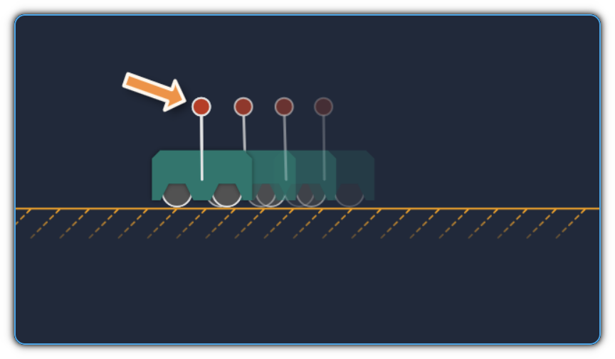
Screenshot of the cart-pole simulator. The “ghost” carts indicate predicted future states produced by the optimization.
The web application is designed to be interactive. This facilitates “poking and prodding” the system to identify unexpected behaviors. Typically when I find an issue, I save a log of the system state to JSON and then load this offline in a Python script (the optimization is also wrapped via nanobind) for further exploration.
Here are some things to try in the sim:
- Click (or touch) to apply external forces to the cart or the pendulum mass. Note that the controller has no external force estimator - the optimization does not explicitly reason about disturbances (the external forces are simply model error).
- Drag the cart set-point slider to steer the cart left and right. This slider adjusts the desired terminal value for $b_x$.
- Toggle the controller off and on to see the system recover from an idle state.
- Adjust the optimization costs:
- For example, set the cost on $b_x$ to zero and observe that the cart can now be pushed back and forth by applying an external force on the pole.
- Alternatively, set the costs on $\theta$ and $\dot{\theta}$ to zero. The system will not longer bother to stabilize the pendulum - but it will continue to track the cart set-point.
Note that not all configurations will be equivalently well-behaved. If the angular rate of the pole gets high enough, the system may explode 💥. If this occurs, reload the page to reset everything.
Conclusions
The first-order conclusion is that this demo was a lot of fun to build. There are a number of improvements I would like to make:
- Add support for the double-pole/pendulum system. Code-generating the dynamics is straightforward, but some tuning of the optimization may be required (+ new code paths for visualization).
- Try out learned methods of stabilization and compare them with the MPC solution.
- Inject more model error into the simulation. At the moment it is a little too perfect (no delay on the control action, for example).
Special thanks to Jack Zhu and Teo Tomić for providing helpful feedback on this project.
References
- Russ Tedrake, Underactuated Robotics, Chapter 10, Trajectory Optimization
- Yang Wang and Stephen Boyd, Fast Model Predictive Control using Online Optimization
- Moritz Diehl, Course Notes: Direct Single and Direct Multiple Shooting
- Sébastien Gros, Mario Zanon, Rien Quirynen, Alberto Bemporad and Moritz Diehl, From linear to nonlinear MPC: bridging the gap via the real-time iteration
- Ettore Pennestrì, Valerio Rossi, Pietro Salvini, Pier Paolo Valentini, Review and comparison of dry friction force models
- Jorge Nocedal, Stephen J. Wright, Numerical Optimization (2nd Edition)